Page No 49:
Question 1:
Explain the concept of a production function.
Answer:
The production function of a firm depicts the relationship between the inputs used in the production process and the final output. It specifies how many units of different inputs are needed in order to produce the maximum possible output. Production function is written as:
Qx = f (L, K)
Where
Qx represents units of output x produced.
L represents units of labour employed.
K represents units of capital employed.
The above equation explains that Qx, units of output x are produced by employing L and K units of labour and capital respectively and by a given technology. As the given level of technology appreciates, the output will increase with the same level of capital and labour units.
Question 2:
What is the total product of an input?
Answer:
Total product is defined as the sum total of output produced by a firm by employing a particular input. It is also known as the Total Physical Product and is represented as
Where, ∑ represents summation of all outputs and Qx represents units of output x produced by an input.
Question 3:
What is the average product of an input?
Answer:
Average product is defined as the output produced by per unit of variable factor (labour) employed. Algebraically, it is defined as the ratio of the total product by units of labour employed to produce the output, i.e.
Where,
TP = Total product
L = units of labour employed
Question 4:
What is the marginal product of an input?
Answer:
Marginal Product is defined as the additional output produced because of the employment of an additional unit of labour. In other words, it is the change in the total output brought by employing one additional unit of labour. Algebraically, it is expressed as the ratio of the change in the total product to the change in the units of labour employed, i.e.
Where,
TPn = Total product produced by employing n units of labour
TPn−1 = Total product produced by employing (n − 1) units of labour
Question 5:
Explain the relationship between the marginal products and the total product of an input.
Answer:
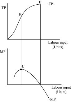
Relationship between marginal products (MP) and the total product (TP) can be represented graphically as
1) TP increases at an increasing rate till point K, when more and more units of labour are employed. The point K is known as the point of inflexion. At this point MP (second part of the figure) attains its maximum value at point U.
2) After point K, TP increases but at a decreasing rate. Simultaneously, MP starts falling after reaching its maximum level at point U.
3) When TP curve reaches its maximum and becomes constant at point B, MP becomes zero.
4) When TP starts falling after B, MP becomes negative.
5) MP is derived from TP by
Question 6:
Explain the concepts of the short run and the long run.
Answer:
Short run:
In short run, a firm cannot change all the inputs, which means that the output can be increased (decreased) only by employing more (less) of the variable factor (labour). It is generally assumed that in short run a firm does not have sufficient or enough time to vary its fixed factors such as, installing a new machine, etc. Hence, the output levels vary only because of varying employment levels of the variable factor.
Algebraically, the short run production function is expressed as
Where,
Qx = units of output x produced
L = labour input
= constant units of capital
Long run:
In long run, a firm can change all its inputs, which means that the output can be increased (decreased) by employing more (less) of both the inputs − variable and fixed factors. In the long run, all inputs (including capital) are variable and can be changed according to the required levels of output. The law that explains this long run concept is called returns to scale. The long run production function is expressed as
Qx = f (L, K)
Both L and K are variable and can be varied.
Question 7:
What is the law of diminishing marginal product?
Answer:
Law of diminishing Marginal Product
According to this law, if the units of the variable factor keeps on increasing keeping the level of the fixed factor constant, then initially the marginal product will rise but finally a point will be reached after which the marginal product of the variable factor will start falling. After this point the marginal product of any additional variable factor will be zero, and can even be negative.
Question 8:
What is the law of variable proportions?
Answer:
Law of Variable Proportions
According to the law of variable proportions, if more and more units of the variable factor (labour) are combined with the same quantity of the fixed factor (capital), then initially the total product will increase but gradually after a point, the total product will start diminishing.
Question 9:
When does a production function satisfy constant returns to scale?
Answer:
Constant returns to scale will hold when a proportional increase in all the factors of production leads to an equal proportional increase in the output. For example, if both labour and capital are increased by 10% and if the output also increases by 10%, then we say that the production function exhibits constant returns to scale.
Algebraically, constant returns to scale exists when
f(nL, nK) = n. f(L, K)
This implies that if both labour and capital are increased by ‘n’ times, then the production also increases by ‘n’ times.
Question 10:
When does a production function satisfy increasing returns to scale?
Answer:
Increasing returns to scale (IRS) holds when a proportional increase in all the factors of production leads to an increase in the output by more than the proportion. For example, if both the labour and the capital are increased by ‘n’ times, and the resultant increase in the output is more than ‘n’ times, then we say that the production function exhibits IRS.
Algebraically, IRS exists when
f(nL, nK) > n. f(L, K)
Page No 50:
Question 11:
When does a production function satisfy decreasing returns to scale?
Answer:
Decreasing returns to scale (DRS) holds when a proportional increase in all the factors of production leads to an increase in the output by less than the proportion. For example, if both labour and capital are increased by ‘n’ times but the resultant increase in output is less than ‘n’ times, then we say that the production function exhibits DRS.
Algebraically, DRS exists when
f(nL, nK) < n. f(L, K)
Question 12:
Briefly explain the concept of the cost function.
Answer:
The functional relationship between the cost of production and the output is called the cost function. It is expressed as
C = f(Qx)
Where,
C = Cost of production
Qx = Units of output x produced
In other words, the output-cost relationship for a firm is depicted by the cost function.
The cost function depicts the least cost combination of inputs associated with different output levels.
Question 13:
What are the total fixed cost, total variable cost and total cost of a firm? How are they related?
Answer:
Total Fixed Cost (TFC)
This refers to the costs incurred by a firm in order to acquire the fixed factors for production like cost of machinery, buildings, depreciation, etc. In short run, fixed factors cannot vary and accordingly the fixed cost remains the same through all output levels. These are also called overhead costs.
Total Variable Cost (TVC)
This refers to the costs incurred by a firm on variable inputs for production. As we increase quantities of variable inputs, accordingly the variable cost also goes up. It is also called ‘Prime cost’ or ‘Direct cost’ and includes expenses like − wages of labour, fuel expenses, etc.
Total Cost (TC)
The sum of total fixed cost and total variable cost is called the total cost.
Total cost = Total fixed cost + Total variable cost
TC = TFC + TVC
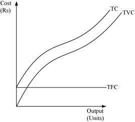
Relationship between TC, TFC, and TVC
1) TFC curve remains constant throughout all the levels of output as fixed factor is constant in short run.
2) TVC rises as the output is increased by employing more and more of labour units. Till point Z, TVC rises at a decreasing rate, and so the TC curve also follows the same pattern.
3) The difference between TC and TVC is equivalent to TFC.
4) After point Z, TVC rises at an increasing rate and therefore TC also rises at an increasing rate.
5) Both TVC and TFC is derived from TC i.e. TC = TVC + TFC
Question 14:
What are the average fixed cost, average variable cost and average cost of a firm? How are they related?
Answer:
Average Fixed Cost:
It is defined as the fixed cost per unit of output.
Where,
TFC = Total fixed cost
Q = Quantity of output produced
Average Variable Cost:
It is defined as the variable cost per unit of output.
Where,
TVC = Total variable cost
Q = Quantity of output produced
Average Cost:
It is defined as the total cost per unit of output. Average cost is derived by dividing total cost by quantity of output.
AC is also defined as the sum total of average fixed cost and average variable cost.
AC = AFC + AVC
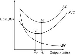
Relationship between AC, AFC, AVC:
1) AVC and AFC are derived from AC as AC = AFC + AVC.
2) The plot for AFC is a rectangular hyperbola and falls continuously as the quantity of output increases.
3) The minimum point of AVC will always exist to the left of the minimum point of AC; i.e., point ‘Z’ will always lie left to point ‘M’.
4) AFC being a rectangular hyperbola falls throughout; this causes the difference between AC and AVC to keep decreasing at higher output levels. However, it should be noted that AVC and AC can never intersect each other. If they intersect at any point, it would imply that AC and AVC are equal at that point. However, this is not possible as AFC will never be zero because it is a rectangular hyperbola that never touches x-axis.
5) AC inherits shape from AVC’s shape and it is because of law of variable proportions that both the curves are U-shaped.
Question 15:
Can there be some fixed cost in the long run? If not, why?
Answer:
No, there cannot be any fixed cost in the long run. In the long run, a firm has enough time to modify factor ratio and can change the scale of production. There is no fixed factor as the firm can change quantity of all the factors of production and therefore there cannot be any fixed cost in the long-run.
Question 16:
What does the average fixed cost curve look like? Why does it look so?
Answer:
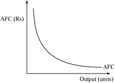
Average fixed cost curve looks like a rectangular hyperbola. It is defined as the ratio of TFC to output. We know that TFC remains constant throughout all the output levels and as output increases, with TFC being constant, AFC decreases.
When output level is close to zero, AFC is infinitely large and by contrast when output level is very large, AFC tends to zero but never becomes zero. AFC can never be zero because it is a rectangular hyperbola and it never intersects the x-axis and thereby can never be equal to zero.
Question 17:
What do the short run marginal cost, average variable cost and short run average cost curves look like?
Answer:
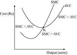
The short run marginal cost (SMC), average variable cost (AVC) and short run average cost (SAC) curves are all U-shaped curves. The reason behind the curves being U-shaped is the law of variable proportion. In the initial stages of production in the short run, due to increasing returns to labour, all the costs (average and marginal) fall. In addition to this in the short run MP of labour also increases, which implies that more output can be produced by per additional unit of labour, leading all the costs curves to fall. Subsequently with the advent of constant returns to labour, the cost curves become constant and reach their minimum point (representing the optimum combination of capital and labour). Beyond this optimum combination, additional units of labour increase the cost, and as MP of labour starts falling, the cost curve starts rising due to decreasing returns to labour.
Question 18:
Why does the SMC curve cut the AVC curve at the minimum point of the AVC curve?
Answer:
SMC curve always intersect the AVC curve at its minimum point. This is because to the left of the minimum point of AVC, SMC is below AVC. SMC and AVC both fall but the former falls at a faster rate. At the minimum point K, AVC is equal to SMC. Beyond K, AVC and SMC both rise but the latter rises at a faster rate than the former and also SMC lies above AVC. Therefore, the only point where SMC and AVC are equal is where SMC intersects AVC, i.e., at the minimum point of the AVC curve.
Question 19:
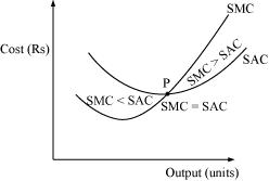
At which point does the SMC curve intersect SAC curve? Give reason in support of your answer.
Answer:
SMC curve intersects SAC curve at its minimum point. This is because as long as SAC is falling, SMC remains below SAC and when SAC starts rising, SMC remains above SAC. SMC intersects SAC at its minimum point P, where SMC = SAC.
Question 20:
Why is the short run marginal cost curve ‘U’-shaped?
Answer:
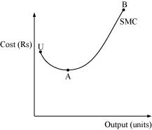
The SMC curve is a U-shaped curve due to the law of variable proportions. In order to understand the reason behind the U-shape of SMC, let us divide the SMC curve (UAB) into three different parts according to the law of variable proportions:
- UA part corresponds to increasing returns to factor.
- Minimum point A corresponds to constant returns to factor.
- AB part corresponds to decreasing returns to factor.
In the initial production stages, the falling part of SMC (UA) is due to application of increasing returns to factor. Then the SMC stops falling and reaches its minimum point ‘A’ due to the existence of constant returns to a factor.
After the minimum point A, SMC starts rising (i.e. ‘AB’ part of SMC) due to the onset of decreasing returns of variable factor. This trend of SMC curve (initially falling, then becoming constant at its minimum point and then rising) makes it look like the English alphabet − ‘U’.
Question 21:
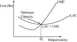
What do the long run marginal cost and the average cost curves look like?
Answer:
The long run marginal cost (LMC) and long run average cost (LAC) are U shaped curves. The reason behind them being U-shaped is due to the law of returns to scale. It is argued that a firm generally experiences IRS during the initial period of production followed by CRS, and lastly by DRS. Consequently, both LAC and LMC are U-shaped curves. Due to IRS, as the output increases, LAC falls due to economies of scale. Then falling LAC experiences CRS at Q1 level of output which is also called the optimum capacity. Beyond Q1 level of output, the firm experiences diseconomies of scale and if the firm continues to produce beyond Q1 level, the cost of production will rise.
Question 22:
The following table gives the total product schedule of labour. Find the corresponding average product and marginal product schedules of labour.
| L | TPL |
| 1 | 15 |
| 2 | 35 |
| 3 | 50 |
| 4 | 40 |
| 5 | 48 |
Answer:
| L | TPL | | |
| − | − | ||
| 1 | 15 | 15 | 15 |
| 2 | 35 | 17.5 | 20 |
| 3 | 50 | 16.67 | 15 |
| 4 | 40 | 10 | − 10 |
| 5 | 48 | 9.6 | 8 |
Question 23:
The following table gives the average product schedule of labour. Find the total product and marginal product schedules. It is given that the total product is zero at zero level of labour employment.
| L | APL |
| 1 | 2 |
| 2 | 3 |
| 3 | 4 |
| 4 | 4.25 |
| 5 | 4 |
| 6 | 3.5 |
Answer:
| L | APL | TPL = AP × L | |
| 1 | 2 | 2 × 1 = 2 | 2 |
| 2 | 3 | 3 × 2 = 6 | 6 − 2 = 4 |
| 3 | 4 | 4 × 3 = 12 | 12 − 6 = 6 |
| 4 | 4.25 | 4.25 × 4 = 17 | 17 − 12 = 5 |
| 5 | 4 | 4 × 5 = 20 | 20 − 17 = 3 |
| 6 | 3.5 | 3.5 × 6 = 21 | 21 − 20 = 1 |
Question 24:
The following table gives the marginal product schedule of labour. It is also given that total product of labour is zero at zero level of employment. Calculate the total and average product schedules of labour.
| L | MPL |
| 1 | 3 |
| 2 | 5 |
| 3 | 7 |
| 4 | 5 |
| 5 | 3 |
| 6 | 1 |
Answer:
| L | MPL | | |
| 1 | 3 | 3 | |
| 2 | 5 | 3 + 5 = 8 | |
| 3 | 7 | 8 + 7 = 15 | |
| 4 | 5 | 15 + 5 = 20 | |
| 5 | 3 | 20 + 3 = 23 | |
| 6 | 1 | 23 + 1 = 24 | |
Question 25:
The following table shows the total cost schedule of a firm. What is the total fixed cost schedule of this firm?
Calculate the TVC, AFC, AVC, SAC and SMC schedules of the firm.
| L | TPL |
| 10 | |
| 1 | 30 |
| 2 | 45 |
| 3 | 55 |
| 4 | 70 |
| 5 | 90 |
| 6 | 120 |
Answer:
| Q (units) | TC (Rs) | TFC = TC − TVC 10 = 10 − 0 (Rs) | TVC = TC − TFC (Rs) | (Rs) | (Rs) | SAC = AFC + AVC (Rs) | SMC = TCn − TCn−1 (Rs) |
| 10 | 10 | 10 − 10 = 0 | − | − | − | − | |
| 1 | 30 | 10 | 30 − 10 = 20 | | | 20 + 10 = 30 | 30 − 10 = 20 |
| 2 | 45 | 10 | 45 − 10 = 35 | | | 17.5 + 5 = 22.5 | 45 − 30 = 15 |
| 3 | 55 | 10 | 55 −10 = 45 | | | 15 + 3.33 = 18.33 | 55 − 45 = 10 |
| 4 | 70 | 10 | 70 − 10 = 60 | | | 15 + 2.5 = 17.5 | 70 − 55 = 15 |
| 5 | 90 | 10 | 90 − 10 = 80 | | | 16 + 2 = 18 | 90 − 70 = 20 |
| 6 | 120 | 10 | 120 − 10 = 110 | | | 18.33 + 1.66 = 19.99 | 120 − 90 = 30 |
Page No 51:
Question 26:
The following table gives the total cost schedule of a firm. It is also given that the average fixed cost at four units of output is Rs 5/-. Find the TVC, TFC, AVC, AFC, SAC and SMC schedules of the firm for the corresponding values of output.
| L | TPL |
| 1 | 50 |
| 2 | 65 |
| 3 | 75 |
| 4 | 95 |
| 5 | 130 |
| 6 | 185 |
Answer:
| Q (units) | TC (Rs) | TFC = Rs 20 (Rs) | TVC = TC − TFC (Rs) | (Rs) | (Rs) | SAC = AFC + AVC (Rs) | SMC = TCn − TCn−1 (Rs) |
| 1 | 50 | 20 | 50 − 20 = 30 | | | 20 + 30 = 50 | 50 − 20 = 30 |
| 2 | 65 | 20 | 65 − 20 = 45 | | | 10 + 22.5 = 32.5 | 65 − 50 = 15 |
| 3 | 75 | 20 | 75 − 20 = 55 | 553=18.33 | | 6.66 + 18.33 = 24.99 | 75 − 65 = 10 |
| 4 | 95 | 20 | 95 − 20 = 75 | | | 5 + 18.75 = 23.75 | 95 − 75 = 20 |
| 5 | 130 | 20 | 130 − 20 = 110 | | | 4 + 22 = 26 | 130 − 95 = 35 |
| 6 | 185 | 20 | 185 − 20 =165 | | | 3.33 + 27.5 = 30.83 | 185 − 130 = 55 |
Question 27:
A firm’s SMC schedule is shown in the following table. The total fixed cost of the firm is Rs 100/-. Find the TVC, TC, AVC and SAC schedules of the firm.
| L | TPL |
| − | |
| 1 | 500 |
| 2 | 300 |
| 3 | 200 |
| 4 | 300 |
| 5 | 500 |
| 6 | 800 |
Answer:
| Q (units) | SMC (Rs) | TFC = Rs 100 (Rs) | (Rs) | TC = TVC + TFC (Rs) | (Rs) | (Rs) |
| − | 100 | − | 100 | − | − | |
| 1 | 500 | 100 | 500 | 500 + 100 = 600 | | |
| 2 | 300 | 100 | 300 + 500 = 800 | 800 + 100 = 900 | | |
| 3 | 200 | 100 | 200 + 800 = 1000 | 1000 + 100 = 1100 | | |
| 4 | 300 | 100 | 300 + 1000 = 1300 | 1300 + 100 = 1400 | | |
| 5 | 500 | 100 | 500 + 1300 = 1800 | 1800 + 100 = 1900 | | |
| 6 | 800 | 100 | 800 + 1800 = 2600 | 2600 + 100 = 2700 | | |
Question 28:
Let the production function of a firm be .
Find out the maximum possible output that the firm can produce with 100 units of L and 100 units of K.
Answer:
− Equation (1)
L = 100 units of labour
K = 100 units of capital
Putting these values in equation (1)
Thus, the maximum possible output that he firm can produce is 500 units.
Question 29:
Let the production function of a firm be Q = 2L2 K2.
Find out the maximum possible output that the firm can produce with 5 units of L and 2 units of K. What is the maximum possible output that the firm can produce with zero unit of L and 10 units of K?
Answer:
a) Q = 2L2 K2 (1)
L = 5 units of labour
K = 2 units of capital
Putting these values in equation (1)
Q = 2 (5)2(2)2
= 2 (25) (4)
Q = 200 units
b) If L = 0 units and K = 100 units
Putting these values in equation (1)
Q = 2 (0)2 (100)2
Q = 0 units
Question 30:
Find out the maximum possible output for a firm with zero unit of L and 10 units of K when its production function is Q = 5L = 2K.
Answer:
Q = 5L + 2K (1)
If L = 0 and K = 10, then putting these values in equation (1)
Q = 5 (0) + 2 (10)
= 20 units of output

